
| Home - Hal and Dee at the Movies | Mail Hal C F Astell - Site Map |
For years my use of Microsoft Office consisted almost entirely of MS Word. Nowadays, however, I'm finding that I hardly use Word at all yet MS Excel proves invaluable many times daily. It would not be a stretch to suggest that certain of my worksheets run my life. My main current project is a book based around an investigation of classic film. While I'm writing the book itself in Word, all the supporting background information is kept in various Excel worksheets.
One of these worksheets keeps a track of the films my wife and I have watched since 2004. Apart from title, director and stars, I'm keeping track of the year of release, our ratings and various statistics to analyse them. As my skills with Excel were not up to the tasks I wished to perform, I have found myself forced to learn much more about how Excel works in order to accomplish them.
I've set this page up for two reasons. Firstly, it'll help to remind myself in the future exactly how I set all this up; and secondly, it may help others who might wish to do some of the same things. In describing how I've configured this worksheet, I'll provide a lesson in nesting functions and conditional formatting. If you have a basic grasp of things already, this may help you to move a step further up the Excel ladder.
Finally, I should point out that I'm using Excel 2000, and while everything I've done here works in that version and in more recent versions, I can't swear that it will all work in previous versions.
While some of what I've set up works across different worksheets in the same file, the source data is in a worksheet called 2004-. It currently runs to over 1,200 lines but the way I've laid it out can be seen from the following image:
The headings are mostly straightforward, but I should explain a few things.
Some fields are split into two for easy sorting. I like to be able to easily sort by director's surname or by film title, without having to worry about words like 'The' or 'A' getting in the way, and thus both Title and Director are split into two.
The 'Add' field is the year that we watched the film. This is so that I can set up statistics to analyse per year. As you can see from the example of The 47 Ronin: Part One, I've watched some films in both 2004 and 2005 and on occasion I've changed my rating on second or third viewing.
As for the ratings themselves, they aren't particularly important for the purposes of this page. However, if you're interested, there is a page that explains my rating system.
I also froze these headings so that they stay on the screen however far I page down through the document. To do this, highlight the line immediately below the headings (ie line 2) and select from the top menu Window then Freeze Panes. When you page down, you'll see the following:

Finally, the reason The Fatal Mallet is in grey is because it's a silent film. This is a simple way for me to keep track of how many silent movies I've watched, but also (after sorting by the year field) how many I've watched that were released after the advent of sound in The Jazz Singer.
You'll notice that in the two screenshots above, our ratings are coloured either blue or red. I used to do this manually, typing in the ratings and then selecting a Font Color of either red or blue from the toolbar. However, conditional formatting makes this much easier by doing the job for me.
I highlighted the entire range that the ratings fall into (currently D2:E1242), then chose Format and then Conditional Formatting from the top menu. I configured these options as follows:

What this means is that if I type either a 1 or a 7 into one of these ratings fields, Excel will automatically change the colour of the font to red. Anything from 2 and 6 inclusive will automatically be changed to blue. Whatever is left remains black, which includes the the hyphens that indicate that either my wife or I watched a particular film while the other didn't, and the occasional NI that shows that we didn't have the faintest idea how to rate a particular film (such as Female Trouble or Guinea Pig 2: Flowers of Flesh and Blood).
Here's where we start playing with formulae, but the initial ones are pretty simple. Below the main body of data, I have a few fields that work out a few statistics that apply to all the films in the list. They look like this:

As you can see, I'm working out a few things here. The top eight fields are pretty straightforward: they simply total up the number of films we've each watched that my wife and I have graded at each individual level in our system, from 7-Classic down to 1-Abysmal, along with the films we found unrateable.
This was done by a simple function called COUNTIF, which counts up the total of fields in a range that satisfy a particular condition. In the case of field D1244 (the first 7-Classic field) the formula looks like this:
=COUNTIF(D2:D1242,7)
D2:D1242 is the range and 7 is the value we're looking at to be included in this count. In other words, this COUNTIF function is going to count up all the instances between D2 and D1242 that equal 7.
One thing to remember here is that to count instances of a particular number Excel requires just the number (like that 7), but to count instances of a particular text string, Excel needs that string enclosed between quotes. Therefore the final unrateable field uses the following slightly different formula:
=COUNTIF(D2:D1242,"NI")
Below these are some basic statistics. The total field simply adds up all the individual totals of ratings (and thus all the films rated); the mean is the average rating of all the films watched by each of us; and the median is the rating that would be in the exact middle if all of our ratings were sorted out and placed in order. These are simple functions for Excel, as follows:
total |
=SUM(D1244:D1251) |
mean |
=AVERAGE(D2:D1242) |
median |
=MEDIAN(D2:D1242) |
Below these statistics are some others that do a similar job with the years these films came out. This time, the range is C2:C1242, thus looking only at year of release. The new function here is the mode, which works out the individual year that appears most often. Again it's a pretty simple function for Excel, as follows:
mean |
=AVERAGE(C2:C1242) |
median |
=MEDIAN(C2:C1242) |
mode |
=MODE(C2:C1242) |
Finally, there are another couple of numbers to explain (the 74 and 108). These work out how many films I've rated higher than my wife (74) and vice versa (108). The problem is that this is far more complex to work out, because Excel assumes that anything is higher than a hyphen. Therefore I'll return to this shortly once I've explained how to nest functions, and thus we'll be able to eliminate any film that wasn't watched by both my wife and I.
The reasons that the above totals were pretty simple to work out is because they applied to all the data in the worksheet. We could just point a function at a range and look at the result. Things only get complex when we start dealing with exceptions, which we'll do now.
Below the totals I've just talked through, I have other totals. These ones look very similar but are restricted to only include films we've watched in a given year. Thus I can see the ratings for films we watched in 2004 and those for 2005. Here's the 2005 set:
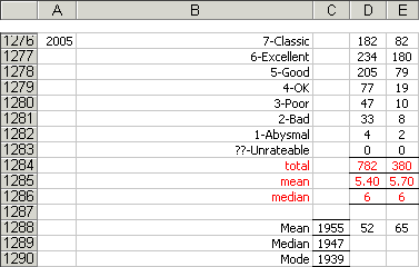
We already know how to count ratings of 7-Classic using a COUNTIF function, but now we need to limit that to just those 7 ratings made in 2005. To do this we have to use something else.
The IF function does something similar to COUNTIF, but it's more flexible. Rather than just counting one for every instance of whatever we're looking for, we can count whatever we like. The IF function checks for a particular result and then returns either one value if it's true or another value if it's false. We can also nest IF functions so that the value if true could be another IF function. Let's look at the formula we'll put in D1276 and then I'll explain how it works.
{=SUM(IF(D2:D1242=7,IF(h2:H1242=2005,1,0),0))}
That's a little daunting. Maybe looking at it this way will make a little more sense:
{=SUM( )}
IF(D2:D1242=7, ,0)
IF(h2:H1242=2005,1,0)
OK, here we go. The SUM function that surrounds everything is easy: it just adds everything up. So what does it add up this time? The answer is everything that is returned true after two nested IF functions.
The first IF function is looking at the range D2:D1242 (my ratings) for any sevens it can find. If it finds one, it moves into the second IF function; if it doesn't, it bypasses that entirely and returns a zero for false.
The second IF function is what takes the place of the true result in the first IF function. It's looking at the range h2:H1242 (the year we watched each film) for the year 2005. If it finds it, it returns a one for true; if not, a zero for false.
So what's happening for each line is that if, and only if, both the D field is a 7 and the H field is 2005, the SUM function counts one. If either the D field isn't a 7 or the H field isn't 2005 or both, it counts zero. What we end up with in field D1276 is the total of all those ones and zeroes added together, and that would be how many films I rated 7 in 2005.
Finally, because nesting these statements makes this count as an array, Excel doesn't require us to just press ENTER when we finish entering the formula. Excel makes us press CTRL-SHIFT-ENTER instead for arrays. Why this is the case I have no idea.
And that's our first array. If that makes sense the rest of the formulae for these totals should make sense too.
Here are the formulae for the ratings:
total |
=SUM(D1277:D1284) |
mean |
{=AVERAGE(IF((h2:H1243=2005),D2:D1243))} |
median |
{=MEDIAN(IF((h2:H1243=2005),D2:D1243))} |
And here are the formulae for the years of release:
mean |
{=AVERAGE(IF((h2:H1243=2005),C2:C1243))} |
median |
{=MEDIAN(IF((h2:H1243=2005),C2:C1243))} |
mode |
{=MODE(IF((h2:H1243=2005),C2:C1243))} |
These formulae cover most of our totals, but not quite all. There's still the 74 and 108 that we put aside earlier: they were the number of times I'd voted higher than my wife and the number of times she'd voted higher than me. I noted then that these were complex formulae, but now we know how to nest functions, they're a bit easier to understand.
To get to that 74, I had to nest quite a few IF functions within a SUM function. How scary does this look?
{=SUM(IF(D2:D1243>E2:E1243,IF(D2:D1243<>"-",IF(E2:E1243<>"-",1,0),0),0))}
Now look at it this way and it should become a bit clearer:
{=SUM( )}
IF(D2:D1242>E2:E1243, ,0)
IF(D2:D1243<>"-", ,0)
IF(E2:E1243<>"-",1,0)
The first IF function is checking to see if each D field is greater than each E field (in other words, whether my ratings were higher than my wife's). If I did outvote my wife, the second and third IF functions make sure that both our fields contain numbers (or more accurately, that they don't contain hyphens, <> meaning 'does not equal').
So, if I vote higher than my wife (the first IF function), my field isn't a hyphen (the second IF function), and her field isn't a hyphen either (the third IF function), then the SUM function counts a one. If any of those IF functions return a false result, then the SUM function counts a zero.
The end result is how many films both my wife and I watched but for which I voted higher. Switching it round to get how many films for which my wife voted higher is as simple as changing that first > sign into a <.
To go one step further and see how many films for which I voted higher in 2005 means adding yet another nested IF function:
{=SUM(IF(D2:D1243>E2:E1243,IF(D2:D1243<>"-",IF(E2:E1243<>"-",IF(h2:H1243=2005,1,0),0),0),0))}
Or, if you want:
{=SUM( )}
IF(D2:D1243>E2:E1243, ,0)
IF(D2:D1243<>"-", ,0)
IF(E2:E1243<>"-", ,0)
IF(h2:H1243=2005,1,0)
To keep a track of how many films I've watched for each year of release, I set up a separate worksheet within the same Excel file. This one is called 'Years' and it looks like this:

This makes it easy for me to see not just how many films I've watched in 1914 or 1967, for instance, but how much I've been concentrating on certain eras, especially the 1930s and the 200s.
The formulae that populate this worksheet are reasonably simple, but they have to look at the main worksheet and there are many of them. Here's the formula to check the range C2:C1246 (the year of release field) in the worksheet called 2004- for the value 1900. The COUNTIF function counts them all up and the hard work here is merely to put in similar formulae into the other 109 cells.
=COUNTIF('2004-'!C2:C1246,1900)
The totals are simple too, being simple SUM functions. The bottom row (row 13) totals up each decade (which corresponds to each column). Field N13 is a grand total that adds up all the decade totals and is thus the total of all films watched. The formulae are:
decade totals |
=SUM(C3:C12) |
grand total |
=SUM(C13:M13) |
Finally, I used conditional formatting to highlight ranges. Because Excel only allows three conditional formats plus the default, I set these numbers of years to be in three different shades of grey, as you can see here:

Just as I set up totals for everything, and then split it up into individual years, I did the same here. The table above counts up the number of films I've watched since I started keeping track of my ratings in 2004. Here's a similar table that only includes films I watched in 2005:

The formulae are more complex because there has to be an IF function built in. Here's the formula for 1900 this time round:
{=SUM(IF('2004-'!C2:C1246=1900,IF('2004-'!h2:H1246=2005,1,0),0))}
What this is doing is using an IF function to look at the C2:C1246 range of the 2004- worksheet for instances of 1900. If it finds one it then looks at the h2:H1246 range for instances of 2005. If that's true too, it returns a 1 and the SUM function adds them all up. Here's a clearer look at the same formula:
{=SUM( )}
IF('2004-'!C2:C1246=1900, ,0)
IF('2004-'!h2:H1246=2005,1,0)
Don't forget to press CTRL-SHIFT-ENTER when entering the formulae because it's an array. This will also put in the curly brackets.
The totals work just as before and so does the conditional formatting.
All of this put together makes a spreadsheet that works as the basis for keeping track of the films I've watched since 2004. It's also taught me plenty about how Excel works and that can't be a bad thing. Maybe it'll help you too. Enjoy.
| Home - Hal and Dee at the Movies | Mail Hal C F Astell - Site Map |